Nuclephile Substitution CH3Cl - SG: Difference between revisions
No edit summary |
|||
| Line 155: | Line 155: | ||
<noinclude> | <noinclude> | ||
== Download == | == Download == | ||
[http://www.vasp.at/vasp-workshop/examples/CH3Cl_SG.tgz CH3Cl_SG.tgz] | |||
{{Template:Molecular dynamics - Tutorial}} | {{Template:Molecular dynamics - Tutorial}} | ||
[[Category:Examples]] | [[Category:Examples]] | ||
Revision as of 08:36, 3 October 2019
Task
In this example the nucleophile substitution of a Cl- by another Cl- in CH3Cl is simulated using a slow growth approach.
Input
POSCAR
   1.00000000000000
     12.0000000000000000    0.0000000000000000    0.0000000000000000
     0.0000000000000000    12.0000000000000000    0.0000000000000000
     0.0000000000000000    0.0000000000000000    12.0000000000000000
C H Cl
   1   3   2
direct
0.53294865 0.56575027 0.49613388
0.53110276 0.65294003 0.50241434
0.44611198 0.52863033 0.51450056
0.58463838 0.52611078 0.55968644
0.32726066 0.74478226 0.64936301
0.57915789 0.51894916 0.36275174
KPOINTS
Automatic
 0
Gamma
 1  1  1
 0. 0. 0.
- For isolated atoms and molecules interactions between periodic images are negligible (in sufficiently large cells) hence no Brillouin zone sampling is necessary.
INCAR
PREC=Low
EDIFF=1e-6
LWAVE=.FALSE.
LCHARG=.FALSE.
NELECT=22
NELMIN=4
LREAL=.FALSE.
ALGO=VeryFast
ISMEAR=-1
SIGMA=0.0516

############################# MD setting #####################################
IBRION=0                                           # MD simulation
NSW=1000                                           # number of steps
POTIM=1                                            # integration step
TEBEG=600                                          # simulation temperature
MDALGO=11                                          # md with Andersen thermostat
ANDERSEN_PROB=0.10                                 # collision probability
LBLUEOUT=.TRUE.                                    # write the BM stuff on the output
INCREM=-1e-4                                       # rate at which CV increases each step
##############################################################################
- The setting LBLUEOUT=.TRUE. tells VASP to write out the information needed for the computation of free energies.
ICONST
R 1 5 0
R 1 6 0
S 1 -1 0
Calculation
In a slow growth simulation, an approximation of the collective variable is increased by the value INCREM every time step. In order for the transformation between the initial and final state to be reversible, the value of INCREM must be infinitesimaly small. In practice we are limited by the desired length of trajectory causing that irreversible rather than reversible work is computed in a slow-growth simulation.
Slow-growth simulations should be considered as an approximate method of free energy calculations whose quality depends strongly on the transformation rate (INCREM). The quality of the simulation can be judged from the hysteresis in the free energy profiles computed for the forward (i.e. reactant -> product) and reverse (i.e. product -> reactant) transformations. Alternatively, free energies can be computed from a series of slow-growth simulations using the Jarzyski identity[1].
The method is most useful as a quick test of the quality of the collective variable before launching any more accurate and time-consuming simulations.
Running the calculation
The mass for hydrogen in this example is set 3.016 a.u. corresponding to the tritium isotope. This way larger timesteps can be chosen for the MD.
For practical reasons, we split our (presumably long) meta dynamics calculation into shorter runs of length of 1000 fs (NSW=1000; POTIM=1). This is done automatically in the script run which looks as follows:
#!/bin/bash

runvasp="mpirun -np x executable_path"

# ensure that this sequence of MD runs is reproducible
cp POSCAR.init POSCAR
cp INCAR.init INCAR
rseed="RANDOM_SEED =         311137787                0                0"
echo $rseed >> INCAR

i=1
while [ $i -le 50 ]
do

  # start vasp
  $runvasp

  # ensure that this sequence of MD runs is reproducible
  rseed=$(grep RANDOM_SEED REPORT |tail -1)
  cp INCAR.init INCAR
  echo $rseed >> INCAR

  # use the last configuration generated in the previous
  # run as initial configuration for the next run
  cp CONTCAR POSCAR

  # backup some important files
  cp REPORT REPORT.$i
  cp vasprun.xml vasprun.xml.$i

  let i=i+1
done
- The user has to adjust the runvasp variable, which holds the command for the executable command.
- Please run this script by typing:
bash ./run
Free energy profile
The following script fgradSG.sh extracts approximate free energy gradients from REPORT.* files obtained in the slow-growth simulation and stores them along with the collectible variables in the file grad.dat:
#!/bin/bash

rm grad.dat

i=1

while [ $i -le 1000 ]
do
  if test -f REPORT.$i
  then
    grep cc REPORT.$i |awk '{print $3}' >xxx
    grep b_m REPORT.$i |awk '{print $2}' >fff
    paste xxx fff >> grad.dat
  fi
  let i=i+1
done

sort -n grad.dat >grad_.dat
mv grad_.dat grad.dat
rm xxx
rm fff
To execute it please type the following:
bash ./fgradSG.sh
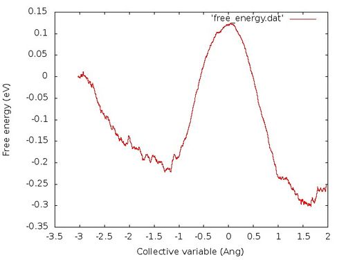
The free energy profile along the collective variable is plotted using the script integrateForward.py:
This script obtains the free energy vs. the collective variable via a simple integration by trapezoid rule. The output is written to standard out so it has to be redirected to a file (we will arbitrarily choose the name free_energy.dat). To execute the script type the following command:
python integrateForward.py grad.dat > free_energy.dat
To plot that script via Gnuplot please use the following:
gnuplot -e "set terminal jpeg; set xlabel 'Collective variable (Ang)'; set ylabel 'Free energy (eV)'; set style data lines; plot 'free_energy.dat'" > free_energy.jpg
The free energy profile should look like the following:
Again this method is only supposed to give a rough estimate for the free energy profile of a material.
References

