H2O molecular dynamics: Difference between revisions
Vaspmaster (talk | contribs) No edit summary |
|||
| (19 intermediate revisions by 2 users not shown) | |||
| Line 1: | Line 1: | ||
{{Template:At_and_mol - Tutorial}} | |||
== Task == | |||
Molecular dynamics calculation for a <math>\mathrm{H}_{2}\mathrm{O}</math> molecule. | |||
== Input == | |||
=== {{TAG|POSCAR}} === | |||
H2O _2 | H2O _2 | ||
0.52918 ! scaling parameter | 0.52918 ! scaling parameter | ||
| Line 29: | Line 20: | ||
1.10 1.43 0.00 T T F | 1.10 1.43 0.00 T T F | ||
the pair correlation function can be visualized using e.g. the following script: | To save time the box size is reduced to 12 a.u. | ||
=== {{TAG|INCAR}} === | |||
{{TAGBL|PREC}} = Normal ! standard precision | |||
{{TAGBL|ENMAX}} = 400 ! cutoff should be set manually | |||
{{TAGBL|ISMEAR}} = 0 ; {{TAGBL|SIGMA}} = 0.1 | |||
{{TAGBL|ISYM}} = 0 ! strongly recommended for MD | |||
{{TAGBL|IBRION}} = 0 ! molecular dynamics | |||
{{TAGBL|NSW}} = 100 ! 100 steps | |||
{{TAGBL|POTIM}} = 1.0 ! timestep 1 fs | |||
{{TAGBL|SMASS}} = -3 ! Nose Hoover thermostat | |||
{{TAGBL|TEBEG}} = 2000 ; {{TAGBL|TEEND}} = 2000 ! temperature | |||
=== {{TAG|KPOINTS}} === | |||
Gamma-point only | |||
0 | |||
Monkhorst Pack | |||
1 1 1 | |||
0 0 0 | |||
== Calculation == | |||
*An example {{TAG|OSZICAR}} file (with 1000 steps and a step size of 0.5 fs) looks like this: | |||
1 T= 2134. E= -.13655511E+02 F= -.14207209E+02 E0=.. EK= 0.55170E+00 SP= 0.00E+00 SK= 0.00E+00 | |||
2 T= 1971. E= -.13643254E+02 F= -.14152912E+02 E0=.. EK= 0.50966E+00 SP= 0.00E+00 SK= 0.00E+00 | |||
3 T= 1336. E= -.13629241E+02 Fd, which just encloses the cutoff sphere corresponding to the plane wave cutoff, is used. This accelerates the calculations by roughly a factor two to three, but causes slight changes in the tot= -.13974630E+02 E0=.. EK= 0.34539E+00 SP= 0.00E+00 SK= 0.00E+00 | |||
4 T= 1011. E= -.13624149E+02 F= -.13885486E+02 E0=.. EK= 0.26134E+00 SP= 0.00E+00 SK= 0.00E+00 | |||
5 T= 1307. E= -.13629772E+02 F= -.13967549E+02 E0=.. EK= 0.33778E+00 SP= 0.00E+00 SK= 0.00E+00 | |||
[[File:Fig H2O 1.png|800px]] | |||
*The pair correlation function can be visualized using e.g. the following script: | |||
*plot_PCDAT | *plot_PCDAT | ||
<pre> | <pre> | ||
awk <PCDAT >PCDAT. | awk <PCDAT >PCDAT.dat ' | ||
NR==8 { pcskal=$1} | NR==8 { pcskal=$1} | ||
NR==9 { pcfein=$1} | NR==9 { pcfein=$1} | ||
| Line 52: | Line 75: | ||
set xlabel "r [Angstrom]" | set xlabel "r [Angstrom]" | ||
set ylabel "g(r)" | set ylabel "g(r)" | ||
plot [0:15] "PCDAT. | plot [0:15] "PCDAT.dat" w lines | ||
! | ! | ||
gnuplot -persist plotfile | gnuplot -persist plotfile | ||
</pre> | </pre> | ||
== Download == | == Download == | ||
[ | [[Media:H2Omd.tgz| H2Omd.tgz]] | ||
{{Template:At_and_mol}} | |||
[[Category:Examples]] | [[Category:Examples]] | ||
Latest revision as of 13:46, 14 November 2019
Overview > O atom > O atom spinpolarized > O atom spinpolarized low symmetry > O dimer > CO > CO vibration > CO partial DOS > H2O >
H2O vibration > H2O molecular dynamics > Further things to try > List of tutorials
Task
Molecular dynamics calculation for a molecule.
Input
POSCAR
H2O _2
0.52918   ! scaling parameter
 12 0 0
 0 12 0
 0 0 12
1 2
select
cart
     0.00     0.00     0.00 T T F
     1.10    -1.43     0.00 T T F
     1.10     1.43     0.00 T T F
To save time the box size is reduced to 12 a.u.
INCAR
PREC = Normal    ! standard precision
ENMAX = 400      ! cutoff should be set manually
ISMEAR = 0 ; SIGMA = 0.1
ISYM = 0         ! strongly recommended for MD
IBRION = 0       ! molecular dynamics
NSW = 100        ! 100 steps
POTIM = 1.0      ! timestep 1 fs
SMASS = -3       ! Nose Hoover thermostat
TEBEG =  2000 ; TEEND = 2000 ! temperature
KPOINTS
Gamma-point only
 0
Monkhorst Pack
 1 1 1
 0 0 0
Calculation
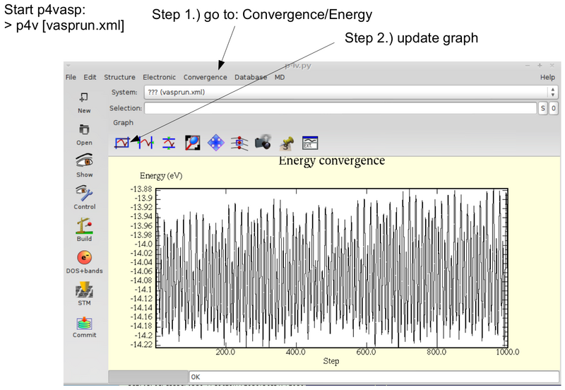
- An example OSZICAR file (with 1000 steps and a step size of 0.5 fs) looks like this:
1 T=  2134. E= -.13655511E+02 F= -.14207209E+02 E0=.. EK= 0.55170E+00 SP= 0.00E+00 SK= 0.00E+00
2 T=  1971. E= -.13643254E+02 F= -.14152912E+02 E0=.. EK= 0.50966E+00 SP= 0.00E+00 SK= 0.00E+00
3 T=  1336. E= -.13629241E+02 Fd, which just encloses the cutoff sphere corresponding to the plane wave cutoff, is used. This accelerates the calculations by roughly a factor two to three, but causes slight changes in the tot= -.13974630E+02 E0=.. EK= 0.34539E+00 SP= 0.00E+00 SK= 0.00E+00
4 T=  1011. E= -.13624149E+02 F= -.13885486E+02 E0=.. EK= 0.26134E+00 SP= 0.00E+00 SK= 0.00E+00
5 T=  1307. E= -.13629772E+02 F= -.13967549E+02 E0=.. EK= 0.33778E+00 SP= 0.00E+00 SK= 0.00E+00
- The pair correlation function can be visualized using e.g. the following script:
- plot_PCDAT
awk <PCDAT >PCDAT.dat '
NR==8 { pcskal=$1}
NR==9 { pcfein=$1}
NR>=13 {
 line=line+1
 if (line==257)  {
    print " "
    line=0
 }
 else
    print (line-0.5)*pcfein/pcskal,$1
}
'
cat >plotfile<<!
# set term postscript enhanced colour lw 2 "Helvetica" 20
# set output "pair_correlation.eps"
set title "pair-correlation of H2O at 2000 K"
set xlabel "r [Angstrom]"
set ylabel "g(r)"
plot [0:15] "PCDAT.dat"  w lines
!
gnuplot -persist plotfile

